Race and Police Related Fatalities

Introduction

I wanted to use data from GitHub maintained by the Washington Post to model whether or not certain races are more likely to be killed by police officers when fatal shootings occur. If so, what factors go into why this is? The relevant data contained information about the time and place of the 3,639 fatal police shootings since the beginning of 2015. It also contained info about the suspects, such as their names and ages, whether or not they were carrying weapons and what weapon they were carrying (the list of weapons includes guns, knives, swords, crossbows, spears, fireworks, bayonets, and more), whether or not the suspect was fleeing and how, the threat level of the suspect (attacking, not attacking, undetermined), whether or not the suspect exhibited signs of mental illness, and of course, the race of the suspect (white, black, Hispanic, Asian, Native American, other, or unknown). It also contained information about whether or not the officer was wearing an active body camera at the time of the shooting.


Inside the Numbers

Taking a look at the data, whites were most often killed by police in the timeframe provided. On average, from 2015 to 2017, 472 whites, 235 blacks, and 167 Hispanics were killed by police per year.

But in a country that is 72.4% white according to the 2010 National Census, perhaps that is to be expected. What would be interesting is to adjust the numbers in the data by the percentage that each demographic comprises in the country. So, that's what I did, but there was one difficult part to this--what to do with the "unknown" race in the data.

I determined that the observations with an unknown race could be dropped as they appeared to be distributed randomly in the dataset. Their average ages as well as the weapons they used, the threats they posed, the states their incidents occurred in, etc. appeared to be close to the averages in the data overall. The assumption that I had to make to justify this decision was that the "unknown" race was just as likely to be white, black, Hispanic, etc. as any other observation. Perhaps that is an assumption worthy of criticism (I could imagine an argument being made that the race of a white person killed is more likely to be identified and made available publicly due to the majority status of whites so that the unknown race observations are more likely to be of minority persuasion), but it was the assumption I deemed best. After dropping these observations, as well as some observations in which age was unknown, I was left with 3,238 data points to work with.

Race	Number times in dataset	Percent of Total in Data	Natl Avg	Ratio: Perc in Data to Natl Avg
Asian	54	1.67%	4.80%	34.74%
Black	825	25.48%	12.60%	202.21%
Hispanic	592	18.28%	16.30%	112.16%
Native Amer	57	1.76%	0.90%	195.59%
Other	34	1.05%	9.30%	11.29%
White	1676	51.76%	72.40%	71.49%

In the table above, the last column gives the percent of each race in the dataset over the percent that particular race makes up of the U.S. as a percent ratio. This means, in practical terms, Asians are 34.74% as likely to be killed by police as we would expect based on the percentage demographic they make up all together in the country and blacks are 202.21% (2 times) more likely based on their percentage. Whites are 71.49% as likely and the other two minority races, Hispanics and Native Americans, are also more likely to have been killed than we would expect by just looking at the percentage of the country's demographic they make up. This seems to confirm what many have contended: given a fatal police shooting has occurred, the suspect is more likely to have been of minority racial persuasion after adjusting for national demographic differences. This does not hold true for the Asian and "other" categories, however.

The next step was determining if I could model the data mathematically to flesh out more insights and how I would do so. I decided to use a logistic regression with two classes (specifically, a Logit model seemed to fit the data best). This required dividing each observation into one of two types and using the other factors recorded in the data to predict if any given observation was one type or another based on the other characteristics. I would then compare my predictions with the actual data to determine how well such modeling works. This is a relatively simple approach that eschews some of the more complicated machine learning techniques that I did not deem necessary for the issue at hand. If I found a model which was better than simply guessing, I could measure the statistical significance of the inputs and use them to explain why certain races are more likely to experience a fatal police shootings than other races.

I decided to divide each observation by a grouping of races of the individuals killed. I wrestled with how this would best be done, and in the end, determined to group by whether or not the suspect was white/Asian or black/Hispanic/Native American/other. I used the information displayed in the table above to help inform this decision, but I also looked at a summary of the data broken down by race to determine which observations were most similar to each other. As well, I used common intuitions to inform this process, and in the end, determined that the split given above made the most sense.


Logistic Modeling and Bias

Using the following inputs:

• Age of suspect
• The state the shooting occurred in
• Whether the suspect was just shot or shot and tasered
• The kind of weapon used
• if the suspect was armed with a ranged weapon (gun, crossbow, etc.)
• If the suspect was using his/her car as a weapon
• If the suspect was not using a weapon
• If the suspect was using a non-ranged weapon
• If the suspect was using a toy weapon
• Whether the suspect displayed signs of mental illness
• Whether the threat level of the suspect was known by officers
• Wheather the suspect was attacking the officer(s)
• Whether the suspect was fleeing
• If the officer was wearing an active body camera
• The gender of the suspect

I wrote a model to determine if I could answer the question at hand. At first, this model gave strange output, and I could not figure out why. Many of the estimations were giving highly non-intuitive results, with states showing dramatically different levels of significance and magnitude in ways one would not expect.

I soon realized that the states with the highest percentage of minorities were also the states most likely to see suspects killed who were black, Hispanic, Native American, or other. This gave a hint that I was not actually capturing any differences across states, but rather, differences in state demographics.

To control for this and "unbias" the models, I took data from the Census Scope online and added it to the model. The code on R I used to scrape this data is given below:

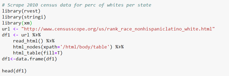
Specifically, I used the percentage of whites in each state to control for demographic differences across the country. Since this data is old and does not account for the percentage of Asians in each state, perhaps there is a better way to control for such demographic differences, but I figured this would be good enough for my purposes. What doesn't matter is that the numbers are exactly correct, but rather, that the variation across states derived from the older dates is consistent with current data. I therefore imagine the better ways of doing this would not make a significant difference in final results, but it definitely would require a lot more work.

I then reran the models and discovered that all data pertaining to states became insignificant after controlling for demographic differences. This means I found no evidence that one's race makes a difference in any given state vs. another when it comes to this issue. I therefore decided to drop state-related variables and focus only on the other factors in the model. This left the model with 14 inputs that I used to predict 1 output--the race group of the individual killed. In the matrix below, we can see how each of these factors correlate with one another ("race_BHNO" meaning whether or not the suspect was black, Hispanic, Native American, or other; "MI_signs" being whether the suspect exhibited signs of mental illness).

For a complete look at each of the variables in the final model, as well as summary statistics, see here.

Model Results

The significant factors determined to be highly indicative of one's race in the model were: 

• The percentage of whites in the given state of the shootings (for reasons already covered)
• The age of the suspect
• Whether the suspect displayed signs of mental illness
• Whether the officer was wearing an active body camera
• The gender of the suspect
• Whether or not the suspect was carrying a "toy weapon" 

In the boxplot below, we can see how age varies from race to race in the dataset, with the two predicted classes being shaded differently. Asians and whites share similar median ages in the data with one another, while the same can be said for blacks, Hispanics, Native Americans, and other.

Returning to the model output, the "intercept" was also very high in the positive direction, meaning that suspects killed by police were much more likely to be black, Hispanic, Native American, or "other race" for reasons not accounted for in the model. We cannot explain why that is by just using the data at hand. The factors that are controlled for in the model, however, have interesting interpretations. If the assumption holds that there are not other factors that significantly affect both the inputs and output of the model, we can use the following interpretations of the statistically significant model estimates to inform our understanding of this subject:

• Percentage of whites in state: As the percentage of non-white people increases per state, the proportion of blacks, Hispanics, Native Americans, and "other race" killed by police increases almost exactly proportionally
• Age: The younger one is when fatally shot by police, the more likely that individual is to be black, Hispanic, Native American, or "other race"
• Signs of mental illness: If the suspect killed by police has exhibited signs of mental illness, he or she is about 49% more likely to have been white or Asian
• Active body camera: If the officer is wearing an active body camera, he/she is 38% more likely to have killed a black, Hispanic, Native American, or "other race" suspect
• Gender: If the suspect killed was male, he was about 50% more likely to have been black, Hispanic, Native American, or "other race"
• Toy weapon: If the suspect killed was brandishing a toy weapon, he/she was about 36% more likely to have been white or Asian

Since this is a "multi-variate" and not a simple logistic regression, we can say that the model interpretations above are in the context of "holding all other factors constant," helping us determine that these relationships are more likely to be causal and not just corollary. In other words, we have good evidence to believe that if all the assumptions of the model hold, these factors are deterministic of why certain races are more likely to be killed in fatal police encounters than others.

Conclusion

Using the data maintained by the Washington Post, I determined that given a fatal police shooting has occurred against a criminal suspect, blacks, Hispanics, and Native Americans are far more likely to have been the ones killed when adjusting for demographic differences in the country. I also determined that age, signs of mental illness, and gender of the suspect are some of the most significant factors in determining this. For a look at the model output, interpretations, accuracy metrics, summary statistics broken down by race, list of weapons, and other information, see here. For a look at the Rscript I used in performing this analysis, see here. Please leave comments if you feel so inclined about what could have been done to make this analysis better, what you liked, etc.

Taking a Statistical Approach to Analyze School Shootings

Introduction

School shootings are ubiquitous in America. What’s as ubiquitous are people’s ideas about why they occur so often and what society can do about it.I had the idea of using statistics to examine this issue. It would be cool if it were possible to use geography and time in order to predict when and/or where the next mass school shooting will occur. Obviously, this could have enormously positive implications. Unfortunately, it's probably an impossible task, given what data is available to do it. There's not a lot of good record keeping when it comes to school shootings--an overabundance of missing values, non-collection of interesting variables, etc. But I did find one dataset that was interesting--a repository on GitHub maintained by the WashingtonPost. I examined this data for many months and what follows are my thoughts on what these data reveal. If you also want to see a machine learning technique called "cluster analysis" used on this data for a more in-depth look into it, see my other post, here.

Exploring the Data

As of August 27, 2018, the dataset contained information on 221 school shootings occurring since (and including) Columbine in 1999. A handful of observations pertaining to specific variables were missing, but for the most part, there was enough to draw meaningful conclusions in a few areas about which I was interested. A precursory exploration of the data revealed some insights that were not surprising, such as:

• 89% of the shootings were known to be committed by a male (or multiple males)
• 61% of the shootings were known to be committed by non-adult aged individuals (usually current or former students)
• 35% of the shootings occurred on a campus where resource officers were present
• 72% of the shootings occurred on campuses where at least 25% of the student-body was eligible for a reduced-priced or free lunch program, indicating a high correlation between poverty and shootings

A look at the final dataset (after I made my manipulations) is available here.

To examine some of the less-obvious results, I needed to decide upon a more-advanced approach. I determined that the most interesting way to do this would be to model and predict the number of casualties in a given school shooting using metrics available in the dataset. Note, this is not to say I would be able to predict anything about when a subsequent school shooting would occur. Rather, I could attempt to answer the question that given a shooting has occurred, what are the factors that lead it to be more or less prejudicial?

Statistical Modeling

There are two ways to approach modeling data in this way—classical statistical modeling (otherwise known as econometrics) and there is machine learning. Machine learning usually produces very good predictions, but it is hard to interpret the model output and it requires a lot of data to be able return reliable predictions (see overfitting). Because I did not have a lot of data at my disposal and I wanted to be able to interpret the model inputs (be able to say that increasing variable x leads to a certain amount of increase or decrease in variable y, etc.), I pursued modeling the data with econometrics.

Econometrics require assuming a distribution--a determination of what the general patterns of the variables in the models are. There were three distributions I tried assuming: normal, Poisson, and negative binomial. Normal distributions are the simplest (think traditional bell curves) but are not always reasonable with real-world data which are usually more complex. For instance, in the dataset at hand, for obvious reasons, casualties can never be negative. They can also never be decimal amounts. When assuming normality, no real number can be excluded from the distribution. For this reason, the normal distribution was most likely not going to be ideal. But that doesn't mean more complex assumptions would be any better. When normality works as well as anything else, it is the best assumption to make because it is so simple.

A Poisson distribution can work well at times when the values of the data being predicted can never be negative or non-integer, as is the case with casualties in this dataset. The Poisson distribution does make one simplifying assumption that can undermine its effectiveness: that the mean of the predicted variable equals its variance. With casualties in this dataset, the variance was much greater than its mean which is why I also decided to model with a negative binomial distribution, correcting for such “overdispersion.” Again, this is not to say the negative binomial distribution will always be better than the Poisson in these cases—the negative binomial assumption is much more complicated, and sometimes the simplest assumptions are the best assumptions.

Running the Models

I modeled casualties using three different models (a model under each distribution assumption), each time with the same 31 inputs, including the gender and age of the shooter, how each weapon was obtained, the weapon type, poverty levels in the school, whether a resource officer was on site, and other such general information. The advantage of using more inputs when modeling is that interpretations of each input are in a context of “holding all other factors constant” (or at least as many other inputs are in the model) which helps the modeler flesh out actual causality and not just correlation. There is a limit though—the more variables used, the wider confidence intervals become on each input’s effect, and it is hard to prove that any of the inputs are statistically significant--you lose degrees of freedom and run into problems pertaining to collinearity. I settled on the inputs I did because, theoretically, each one seemed like it could add something of value to the model and would have an interesting interpretation. See the data’s summary statistics for information about each input.

The negative binomial model worked best. I determined this by creating the following function on R to derive the model log likelihood, AIC, and BIC (these three metrics together are known as the information criteria):

Running these lines of code, I extracted each model’s information criteria:

Information criteria is a general indication of residual dispersion in the fitted models—how well the model predictions fit the data. The higher the value of the log likelihood, the better the model performs. The lower the values of the AIC and BIC, the same can be said. In effect, these are three different methods to capture the same general information, and while they do not always agree with one another, in this case, they did. It was easy to determine that the negative binomial model (NB) fit best on the given data.

Meaningful Insights

Resource Officer – Using the superior NB model as the standard for deriving results, interpreting most of what the model returned was fairly intuitive (example - when a shooting is indiscriminate such as the case of Sandy Hook, Columbine, and Stoneman Douglas, more casualties can be expected than from an accidental shooting). But there were some surprises as well. For one thing, the data highly suggested that the greater the percentage of students eligible for the reduced-priced lunch program, the fewer casualties occur per school shooting, holding all else constant. The opposite can be said about if a resource officer is on campus—when a resource officer is on campus during a shooting, more casualties occur, all else constant (on average, 3.5 more). Not only that, but both the resource officer and the school lunch variables were some of the most significant inputs in the model—we can be very confident that these effects were not measured by chance. Also, because there were many other inputs in the model, we can say that other potentially corollary factors were held constant, further suggesting causal relationships.

Many times, we assume the more poverty in a school, the more violence. We can also think that having a resource officer on campus will shut down a shooter more quickly before many casualties have occurred. But the data suggest otherwise. This was a finding I was surprised to find. In the cases where results are unexpected like this, I would like to see these results replicated in another study. But it may simply be that our intuition needs to change when thinking about the effects of a resource officer and poverty in schools. Also worthy of being noted, every model I ran seemed to suggest this same general relationship and statistical significance.

Weapon Type – In most cases, the model suggested that the weapon used in the shooting makes a significant difference in the number of casualties. In particular, the most statistically significant input pertaining to weapon type was “rifle,” which denotes any kind of rifle (assault or otherwise) used in the shooting. According to the model, rifles cause on average 6 more casualties when used in a school shooting compared to when some other weapon is used. This may be due to one-off school shooting events where a handful of particular dangerous shooters just happened to use a rifle, but again, the variable was very statistically significant, so to make the claim that rifles do not cause any more casualties in a school shooting than any other weapon, some compelling reason would have to be offered.

Illegally Obtained Weapons – As soon as I saw that the data had an indicator of whether or not the weapon used in the shooting was obtained illegally, I wanted to know what it had to say about casualties. When modeling this, the data seemed to show that fewer casualties were caused when a weapon was obtained illegally. It should be noted that this input was statistically insignificant (meaning we either need new data or a different study to draw any meaningful inferences from how the illegality of a weapon affects casualties). Nevertheless, the relationship seemed to be suggestive of fewer casualties (or at least the same number of casualties) when an illegally obtained weapon is used vs. a legally obtained weapon.

 

Wrapping Up

For a complete look at the code I used (all on R) to produce this analysis, see here. For a complete look at the final negative binomial model output and its interpretations, see here. Although the data used in this analysis proved to have limitations, it still revealed insights that were not obvious and were intriguing. I would like to obtain other data in different formats (ideally without any missing values) to perform other analyses to further validate or invalidate these findings. For now, the insight that having a resource officer on campus leads to more school shootings was interesting. A campus which is generally more impoverished (as indicated by the campuses with the highest percentages of students eligible for reduced-priced lunch) saw fewer casualties per school shootings, even when other factors were held constant. I did not expect either of these findings and found such discoveries fascinating.